Preface
This article does not involve complicated mathematical formulas as much as possible, and describes the core points of the model frequently asked in the interview in a language that is relatively easy to understand but not professional.
I hope that I can help you to review the core content of the review when you are looking for a job, or to grasp the focus of each model in the process of preparation.
Practical environment description:
Python 2.7;
Sklearn 0.19.0;
Graphviz 0.8.1 Decision Tree Visualization.
First, the decision tree
▌1.1 Principle
As the name implies, the decision tree uses a tree to represent our entire decision-making process. This tree can be a binary tree (such as CART can only be a binary tree) or a multi-fork tree (such as ID3, C4.5 can be a multi-fork tree or a binary tree).
The root node contains the entire sample set, and each leaf node corresponds to a decision result (note that different leaf nodes may correspond to the same decision result), and each internal node corresponds to a decision process or an attribute test. The path from the root node to each leaf node corresponds to a decision test sequence.
for example:
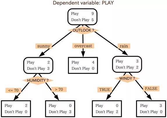
Like the example above, the training set consists of three characteristics: outlook (weather), humidity (humidity), and windy (whether there is wind).
So how do we choose features to divide the training set? How is the threshold for the classification of continuous features (such as humidity) determined?
The generation of decision trees is to continuously select the optimal features to divide the training set, which is a recursive process. There are three conditions for recursive return:
(1) The samples contained in the current node belong to the same category and do not need to be divided;
(2) The current attribute set is empty, or all samples have the same value on the attribute set and cannot be divided;
(3) The current node contains a sample set that is empty and cannot be divided.
1.2 ID3, C4.5, CART
These three are very famous decision tree algorithms. Simple and rude, ID3 uses information gain as a criterion for selecting features; C4.5 uses information gain ratio as a criterion for selecting features; CART uses the Gini index as a criterion for selecting features.
ID3
Entropy represents the amount of information contained in the data. The smaller the entropy, the higher the purity of the data, that is, the more consistent the data, which is what each child node looks like after we divide it.
Information gain = pre-division entropy - entropy after partitioning. The greater the information gain, the greater the “purity increase†obtained by using the attribute a to divide. That is to say, the training set is divided by the attribute a, and the obtained result is relatively high in purity.
ID3 only applies to the two-category problem. ID3 can only handle discrete attributes.
C4.5
C4.5 overcomes the problem that ID3 can only deal with discrete attributes, and the problem that information gain biases to select more features, and uses information gain ratio to select features. Information gain ratio = information gain / pre-division entropy The information gain ratio is selected as the optimal feature.
C4.5 To process continuous features, the feature values ​​are first sorted, and the intermediate values ​​of two consecutive values ​​are used as the dividing criteria. Try each division and calculate the corrected information gain, and select the split point with the largest information gain as the split point of the attribute.
CART
CART differs from ID3, C4.5 in that the tree generated by CART must be a binary tree. That is to say, whether it is regression or classification problem, whether the feature is discrete or continuous, whether the attribute has multiple or two values, the internal node can only make two points according to the attribute value.
The full name of CART is the classification and regression tree. From this name, you should know that CART can be used for both classification and regression problems.
In the regression tree, the square error minimization criterion is used to select features and divide them. The predicted value given by each leaf node is the mean of all sample target values ​​divided into the leaf nodes, thus minimizing the squared error for a given partition.
To determine the optimal score, it is also necessary to traverse all the attributes, and all their values ​​to try to divide and calculate the least square error in this case, and select the smallest as the basis for this division. Since the regression tree generation uses the square error minimization criterion, it is also called the least squares regression tree.
Classification tree species, using Gini index minimization criteria to select features and divide them;
The Gini index indicates the uncertainty of the set, or is not pure. The larger the Gini index, the higher the set uncertainty and the greater the purity. This is similar to entropy. Another way to understand the Gini index is that the Gini index is designed to minimize the probability of misclassification.
▌1.3 information gain vs information gain ratio
The introduction of the information gain ratio is due to a disadvantage of information gain. That is: the information gain is always biased towards choosing attributes that take more values. The information gain ratio adds a penalty to this and solves this problem.
▌1.4 Gini index vs entropy
Since both of these can represent the uncertainty of the data, the purity is not. So what is the difference between the two?
The calculation of the Gini index does not require logarithmic operations and is more efficient;
The Gini index is more biased towards continuous attributes, and entropy is more biased toward discrete attributes.
▌1.5 pruning
Decision tree algorithms are easy to overfitting. Pruning algorithms are used to prevent over-fitting of decision trees and improve the performance of pan-China.
Pruning is divided into pre-pruning and post-pruning.
Pre-prune refers to the evaluation of each node before the division in the decision tree generation process. If the current division does not bring about the generalization performance improvement, the division is stopped, and the current node is marked as a leaf node.
Post-prune refers to first generating a complete decision tree from the training set, and then examining the non-leaf nodes from the bottom up. If the corresponding subtree is replaced by a leaf node, the generalization performance can be improved. Replace the subtree with a leaf node.
So how do you judge whether the generalization performance is improved? The easiest way to do this is to leave a portion of the data as a validation set for performance evaluation.
▌1.6 Summary
The decision tree algorithm mainly includes three parts: feature selection, tree generation, and tree pruning. Common algorithms are ID3, C4.5, and CART.
Feature selection. The purpose of feature selection is to select features that can be classified into training sets. The key to feature selection is the criteria: information gain, information gain ratio, Gini index;
The generation of a decision tree. It is usually the criterion that the information gain is the largest, the information gain ratio is the largest, and the Gini index is the smallest. Starting from the root node, recursively generates a decision tree. Equivalent to continuously selecting local optimal features, or dividing the training set into subsets that can be correctly classified;
The pruning of the decision tree. The pruning of the decision tree is to prevent over-fitting of the tree and enhance its generalization ability. Includes pre-pruning and post pruning.
Second, random forest (Random Forest)
To say that random forests must first say Bagging, to say that Bagging must first talk about integrated learning.
▌2.1 Integrated learning method
Ensemble learning accomplishes learning tasks by building and combining multiple learners. Integrated learning often combines multiple learners to achieve superior generalization performance over a single learner.
According to whether the individual learners are the same type of learners (generated by the same algorithm, such as C4.5, BP, etc.), they are divided into homogeneity and heterogeneity. A homogenous individual learner is also called a base learner, and a heterogeneous individual learner is directly an individual learner.
Principle: To achieve better performance than a single learner, individual learners should be different and different. That is, individual learners should have certain accuracy, can not be worse than weak learners, and have diversity, that is, there are differences between learners.
According to the generation method of individual learners, integrated learning is divided into two categories:
There is a strong dependency between individual learners and a serialization method that must be generated serially. The representative is Boosting;
There is no strong dependency between individual learners, and parallelization methods that can be generated simultaneously. The representative is Bagging and Random Forest.
▌2.2 Bagging
As mentioned earlier, individual learners should be independent in order to achieve improved performance. Although “independence†is often not possible in real life, it can be managed to make the base learner as large as possible.
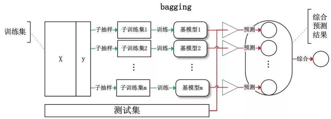
The approach given by Bagging is to sample the training set, produce several different subsets, and train a base learner from each training subset. Due to the different training data, our base learners are expected to have large differences.
Bagging is a representative of parallel integrated learning methods. The sampling method is self-sampling, which uses sampling that is put back. Approximately 63.2% of the data in the initial training set appeared in the sampling set.
Bagging uses simple voting for classification problems and simple averaging for regression problems.
Bagging advantages:
Efficient. The Bagging integration is the same as the complexity of the direct training based learner;
Bagging can be applied to multi-classification and regression tasks without modification.
Outsourcing estimates. Use the remaining samples as a validation set for an out-of-bag estimate.
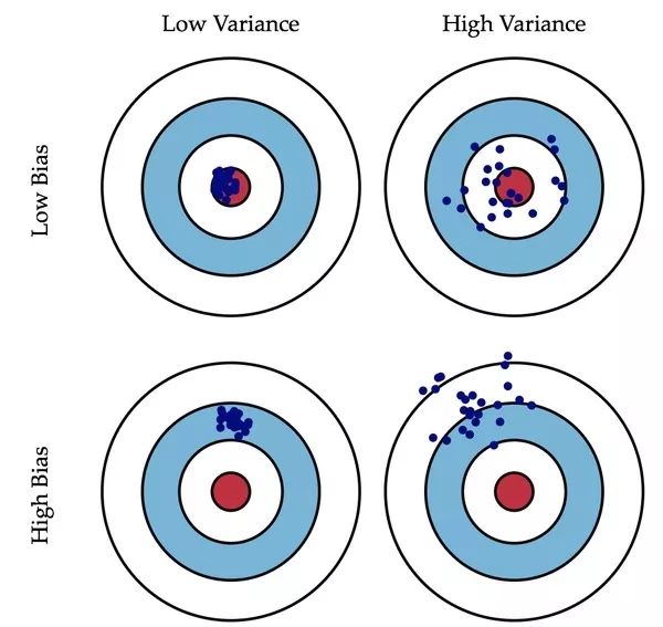
Bagging focuses on reducing variance. (low variance)
▌2.3 Random Forest (Random Forest)
2.3.1 Principle
Random Forest is a variant of Bagging. Based on the decision tree-based learning device to build Bagging integration, Ramdon Forest further introduces random attribute selection in the decision tree training process.
The original decision tree selects the optimal attribute from all the attributes. Each node in each decision tree of Ramdom Forest randomly selects a subset of K attributes from the attribute set of the node, and then selects the optimal attribute from the subset of attributes to divide.
K controls the degree of introduction of randomness and is an important hyperparameter.
Forecast:
Classification: simple voting method;
Regression: Simple average method.
2.3.2 Advantages and disadvantages
advantage:
Since each attribute is no longer considered, but a subset of attributes, the computational efficiency is lower than that of Bagging, and the training efficiency is higher;
Due to the increased perturbation of the properties, the performance of the base learner in the random forest is reduced, which makes the performance of the random forest in the beginning poor, but with the increase of the base learner, the random forest usually converges to the lower generalization error. Compared to Bagging;
The introduction of two randomness makes the random forest not easy to fall into over-fitting and has good anti-noise ability;
Adaptable to data, can handle discrete and continuous, no need to standardize;
The importance of the variable can be obtained, based on the oob misclassification rate and the change based on the Gini coefficient.
Disadvantages:
It is easy to overfit when the noise is large.
Third, AdaBoost
AdaBoost is the representative of Boosting. Earlier we mentioned that Boosting is a very important type of serial learning method in integrated learning.
▌3.1 Boosting
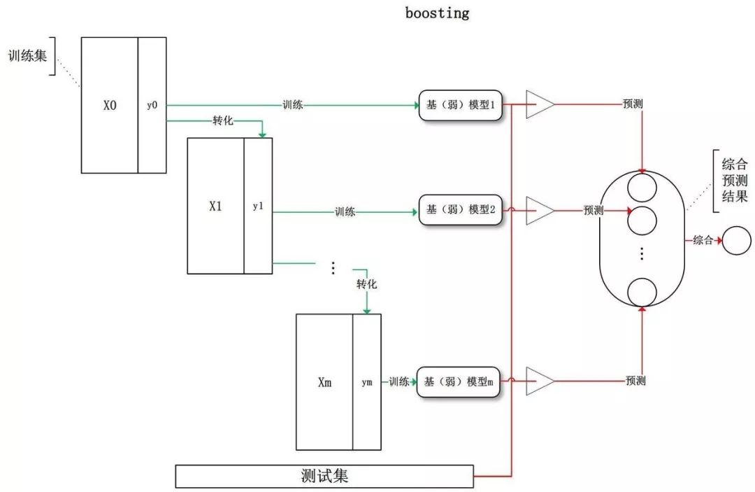
Boosting refers to an integrated learning method in which individual learners have strong dependencies and must be serially serialized. His source of thought is the top of the three smugglers. Boosting means improvement, which means that you want to promote each weak learner to a strong learner.
The working mechanism is as follows:
First learn a base learner from the initial training set;
Adjusting the distribution of training samples according to the performance of the base learner, so that the training samples that the previous base learner made a mistake receive more attention in the following;
Training the next base learner based on the adjusted sample distribution;
This is repeated until the number of base learners reaches T, and the T base learners are finally weighted and combined.
The adjustment of the training sample distribution is mainly to increase the weight of the correctly classified samples by increasing the weight of the misclassified samples.
Boosting focuses on reducing bias. (low bias)
▌3.2 AdaBoost principle
Face two problems:
(1) In each round, how to change the probability distribution or weight distribution of the training data. (It can also be resampled, but AdaBoost doesn't do this);
(2) How to combine weak classifiers into strong classifiers.
AdaBoost's approach:
(1) Improve the weights of the samples misclassified by the previous round of weak classifiers, and reduce the weights of those samples that are correctly classified. In this way, those data that are not correctly classified are subject to the attention of the latter round of weak classifiers due to their increased weight;
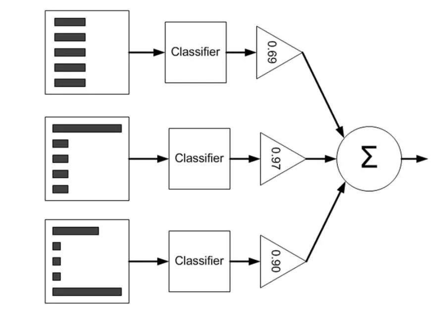
(2) Adopt a weighted majority vote. Specifically, the weight of the classifier with a low classification error rate is increased, so that it plays a larger role in the voting, and the weight of the weak classifier with a large classification error rate is reduced, so that it plays a smaller role in the voting.
Weak classifiers are linearly combined into a strong classifier.
Training objectives:
Minimize the exponential loss function.
Three parts:
(1) classifier weight update formula;
(2) The sample distribution (that is, the sample weight) update formula;
(3) Additive model. Minimize the exponential loss function.
▌3.3 AdaBoost Advantages and Disadvantages
advantage:
Without changing the given training data, the weight distribution of the training data is constantly changed, so that the training data plays a different role in the learning of the basic classifier. This is a feature of AdaBoost;
Building a final classifier using a weighted linear combination of basic classifiers is another feature of AdaBoost;
AdaBoost has been proven to be a good way to prevent overfitting, but so far it has not been theoretically proven.
Disadvantages:
AdaBoost is only available for two-category issues.
Fourth, GBDT
GBDT (Gradient Boosting Decision Tree) is also called MART (Multiple Additive Regression Tree). It is an iterative decision tree algorithm.
This article describes the following aspects:
Regression Decision Tree(DT);
Gradient Boosting (GB);
Shrinkage (an important evolutionary branch of the algorithm, most of the source code is currently implemented based on this version);
GBDT scope of application;
Contrast with random forests.
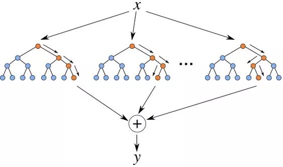
▌4.1 DT: Regression Tree Regression Decision Tree
The trees in GDBT are all regression trees, and the core is the result of accumulating all the trees as the final result. It only makes sense to add up the results of the regression tree, and the result of the classification is meaningless.
The GDBT adjustment can be used to classify the problem, but the internal is still a regression tree.
This part is the same as in the decision tree, nothing more than feature selection. The regression tree uses the minimum mean square error, and the classification tree uses the minimum Gini index (CART).
▌4.2 GB: Gradient iteration Gradient Boosting
First of all, Boosting is an integrated approach. A strong classifier is obtained by combining weak classifiers, which is serial, and several weak classifiers are sequentially trained. The core of GBDT is that each tree learns the residuals of all previous tree conclusions.
Gradient is reflected in: whether the cost function of the previous tree is the mean square error or the mean difference, as long as it is measured by error, then the residual vector is its global optimal direction, which is the Gradient.
▌4.3 Shrinkage
Shrinkage is an important evolutionary branch of the GBDT algorithm, and most of the source code is currently based on this version.
The core idea is that Shrinkage believes that each time a small step is taken to approximate the results, it is easier to prevent overfitting than the way that a large step is approached quickly.
In other words, it does not trust the residuals that are learned each time. It believes that each tree only learns a small part of the truth. When accumulating, only a small part is accumulated, and more trees are used to make up for the shortcomings.
The specific approach is: still use the residual as the learning goal, but for the result of the residual learning, only a small part (step* residual) is gradually added to the target, and the step is generally small 0.01-0.001, resulting in each tree. The residual is a gradual change rather than a steep one.
Essentially, Shrinkage sets a weight for each tree, multiplying it by the weight, but not with Gradient.
This weight is step. Like AdaBoost, Shrinkage is also empirically proven to reduce overfitting, and there is no theoretical proof.
▌4.4 GBDT Scope of application
GBDT can be applied to regression problems (linear and nonlinear), compared to logistic regression, which can only be used for linear regression, and GBDT is more widely applicable;
GBDT can also be used for two-category problems (set thresholds, greater than positive, otherwise negative) and multi-classification problems.
▌4.5 GBDT and random forest
The same point between GBDT and random forest:
Are composed of multiple trees;
The final result is determined by multiple trees.
Differences between GBDT and random forests:
The composition of random forests can be classification trees and regression trees; the composition of GBDT can only be a regression tree;
The trees that make up the random forest can be generated in parallel (Bagging); GBDT can only be generated serially (Boosting);
For the final output, the random forest uses a majority vote or a simple average; while the GBDT accumulates all results, or weights up;
Random forests are not sensitive to outliers, and GBDT is very sensitive to outliers;
The random forest has the same weight as the training set, and the GBDT is the integration of weak classifiers based on weights;
Random forests improve performance by reducing the variance of the model, and GBDT improves performance by reducing model bias.
TIP
1. What are the advantages of GBDT compared to decision trees?
Generalization performance is better! The biggest advantage of GBDT is that the residual calculation at each step actually increases the weight of the fault-corrected samples in disguise, while the samples that have been paired tend to zero. This will focus more on the samples of the faults.
2. Where is Gradient reflected?
It can be understood that the residual is the globally optimal absolute direction, similar to the gradient.
3. re-sample
GBDT can also introduce Bootstrap re-sampling while using residuals. This option was introduced in most implementations of GBDT, but whether it must be used or not.
The reason is the randomness caused by re-sample, which makes the model non-reproducible, and poses certain challenges for the evaluation, such as it is difficult to determine whether the performance improvement is due to the feature or the random factor of the sample.
Five, Logistic regression
LR principle;
Parameter Estimation;
Regularization of LR;
Why is LR better than linear regression?
The relationship between LR and MaxEnt.
▌5.1 Principle of LR model
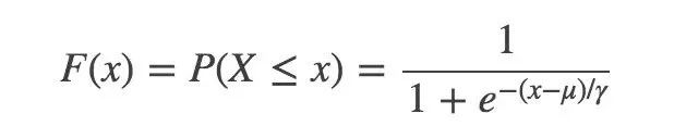
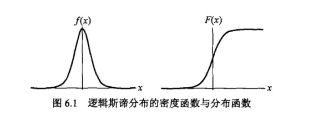
First you must give the Logistic distribution:
u is the positional parameter and r is the shape parameter. The symmetry point is (u, 1/2), and the smaller r is, the steeper the function is near u.
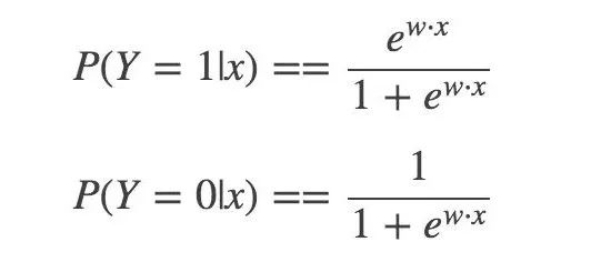
Then, the two-class LR model is a parameterized logistic distribution, expressed using conditional probability:
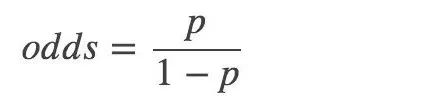
Then, the odds of an event (odds): the ratio of the probability of occurrence of the event to the non-occurrence:
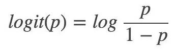
Logarithmic probability:
Then for logistic regression, the logarithmic probability of Y=1 is:
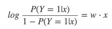
Finally, the log probability of outputting Y=1 is a model of the linear function of the input x, which is the logistic regression model.
▌5.2 Parameter estimation
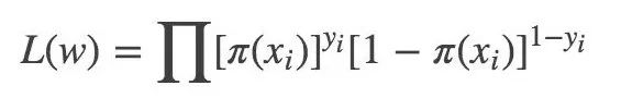
In statistics, maximum likelihood estimation is often used to estimate parameters. That is, a set of parameters is found, so that the likelihood (probability) of our data is the largest under this set of parameters.
Likelihood function:
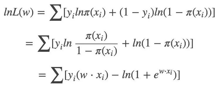
Log likelihood function:
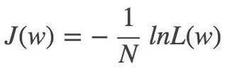
Corresponding loss function:
▌ 5.3 Optimization method
In the parameter estimation of the logistic regression model, the last is to find the minimum value for J(W). This optimization problem without constraints is usually solved by gradient descent or Newton method.
Solving Logistic Regression Parameter Estimation Using Gradient Descent Method
Find the J(W) gradient: g(w):
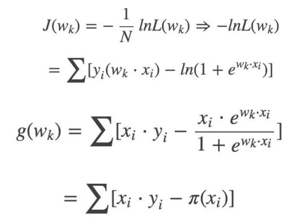
Update Wk:
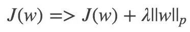
$$ W_{k+1} = W_k - \lambda*g(W_k) $$
▌5.4 Regularization
Regularization is to solve the overfitting problem. It is divided into L1 and L2 regularization. The model complexity assessment is added mainly by correcting the loss function;
Regularization is in line with the Occam razor principle: in all possible models, the well-known data can be interpreted very well and the simplest is the best model.
The p-table examples, p=1 and p=2 apply the L1 and L2 regulars, respectively.
L1 regularization. The sum of the absolute values ​​of the elements in the vector. Also known as the Lasso regularization. The key is to enable automatic selection of features, and parameter sparsity can avoid noise introduced by non-essential features;
L2 regularization. Make each element as small as possible, but not zero. In the regression, someone called his return called Ridge Regression, and some called him "weight decay."
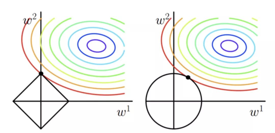
A summary of the sentence is: L1 tends to produce a small number of features, while other features are 0, and L2 will select more features, these features will be close to 0.
▌5.5 Logistic Regression vs Linear Regression
First, logistic regression is better than linear regression.
Both belong to a generalized linear model.
Linear regression optimizes the least squares method for objective functions, while logistic regression uses maximum likelihood estimates. Logistic regression is based on linear regression, mapping the weighted sums through the sigmoid function to the space within the 0-1 range.
Linear regression is predicted over the entire real range, with consistent sensitivity, and the classification range needs to be [0, 1]. Logistic regression is a regression model that reduces the prediction range and limits the prediction to [0,1].
The logic curve is very sensitive at z=0, and is not sensitive at z>>0 or z<<0, limiting the predicted value to (0,1). The robustness of logistic regression is better than linear regression.
▌5.6 Logistic Regression Model vs Maximum Entropy Model MaxEnt
Simple and rude: Logistic regression is not fundamentally different from the maximum entropy model. Logistic regression is a special case when the maximum entropy corresponds to the second class, that is, when the logistic regression is extended to multiple categories, it is the maximum entropy model.
Principle of Maximum Entropy: When learning the probability model, the model with the largest entropy is the best model among all possible probability models (distributions).
Six, SVM support vector machine
Although our goal is not to involve formulas as much as possible, there is no way to refer to SVMs that do not involve formula derivation, because the most basic and difficult question in the interview is to ask SVM, the mathematical formula for the dual problem of SVM is derived. .
Therefore, if you want to learn machine learning well, you still have to collapse your heart. It is not only necessary to master the core ideas of the principle, but also to learn the formula.
▌6.1 SVM principle
Simply and rudely: The idea of ​​SVM is to find a hyperplane to correctly classify the data set. For data that is inseparable from existing dimensions, the kernel function is mapped to the high-latitude space to make it linearly separable.
Support Vector Machine SVM is a two-class model. Its basic model is the linear classifier that defines the largest interval in the feature space. The maximum interval makes it different from the perceptron. The SVM learning strategy is to maximize the interval and can be formalized to solve convex quadratic programming problems.
SVM is divided into:
Linear separable support vector machines. A linear classifier learned through the hard interval maximization when the training data is linearly separable;
Linear support vector machine. A linear classifier learned by maximizing the soft interval when the training data is approximately linearly separable;
Nonlinear support vector machine. When the training data is linearly inseparable, the nonlinear support vector machine is learned by using kernel techniques and soft interval maximization.
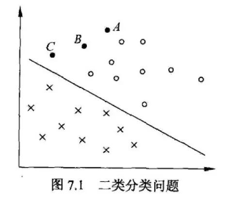
In the figure above, X is a negative example and O is a positive example. The training data at this time can be divided, and the linear separable support vector machine corresponds to a straight line that correctly divides the two types of data and has the largest interval.
6.1.1 Support Vectors and Intervals
Support Vector: In the case of linear separability, an instance of a sample point in the sample point of the training data sample set that is closest to the separated hyperplane is called a support vector.
The function interval is defined as follows:
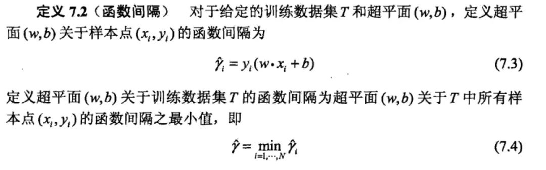
Yi represents the target value, which is +1, -1. The function interval can indicate the accuracy and confidence of the classification prediction. But there is a bad property: as long as the W and B are changed in multiples, although the hyperplane does not change at this time, the function interval will become larger.
So we thought of applying some constraints on the hyperplane's normal vector W, such as normalization, so that the interval is determined, which leads to geometric spacing:
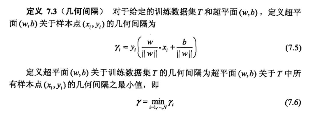
The basic idea of ​​support vector learning is to solve the classification hyperplane that can correctly divide the training data set and has the largest geometric interval.
6.1.2 Dual problem
In order to solve the optimization problem of linear separable support vector machine:
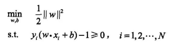
As the original optimization problem, the Lagrangian duality is applied, and the optimal solution of the original problem is obtained by solving the dual problem. This is the dual algorithm of the linear separable support vector machine.
The original algorithm can also solve SVM, but the reason to solve it with dual problem is:
First, dual problems are often easier to solve;
The second is the natural introduction of the kernel function, which is then extended to the nonlinear classification problem.
Speaking a bit off topic, this is also a question that will be asked during the interview: since the original problem can be solved, why should it be converted into a dual problem?
The answer is the above two points. Due to the length of the text, the derivation of mathematical formulas is not here. You can refer to Machine Learning and Statistical Learning Methods.
6.1.3 Kernel function
For problems that are inseparable in the original space, it is linearly separable in high dimensional space.
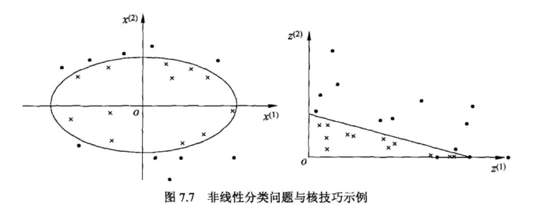
For linearly inseparable problems, the kernel function can be used to map from the original space to the high-latitude space, making the problem linearly separable. The kernel function can also cause the inner product computed in high dimensional space to be done by a function in a low dimensional space.
Commonly used kernel functions are: Gaussian kernel, linear kernel, polynomial kernel.
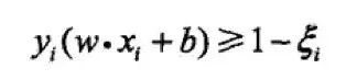
6.1.4 Soft interval
Support vector machine learning methods for linear separable problems are not applicable to current non-separable training data. Therefore, the interval function is modified to a soft interval, and for the function interval, a slack variable is added thereto so as to satisfy greater than or equal to 1. The constraint becomes:
▌ 6.2 Advantages and disadvantages
Disadvantages:
Time and space overhead is relatively large and training time is long;
The selection of the kernel function is difficult, mainly based on experience.
advantage:
Good results are often obtained on small training sets;
Using a kernel function avoids the complexity of high latitude space;
Strong generalization ability.
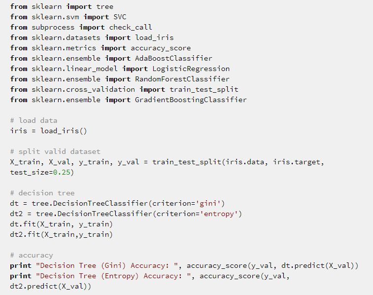
Seven, use sklearn for actual combat
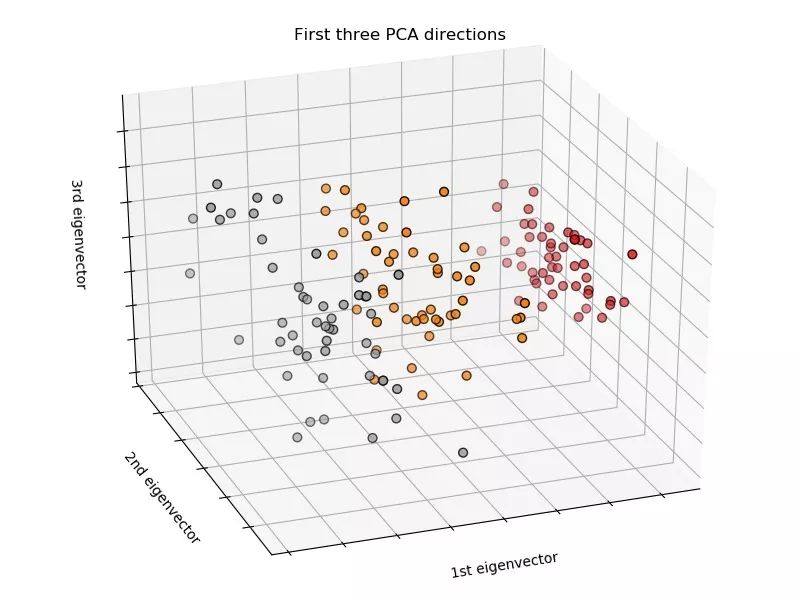
Use sklearn to use the decision tree to divide the Iris flower dataset. There is no fixed random seed on the code, so the result of each run will be slightly different.
Dataset 3D visualization:
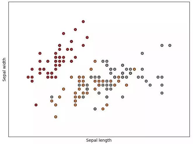
Visualization on Sepal length and Sepal width 2D:
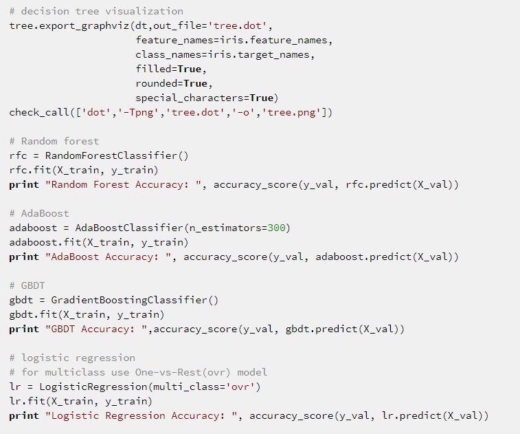
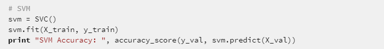
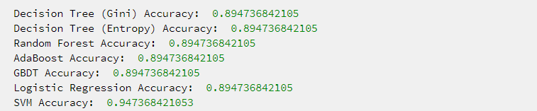
operation result:
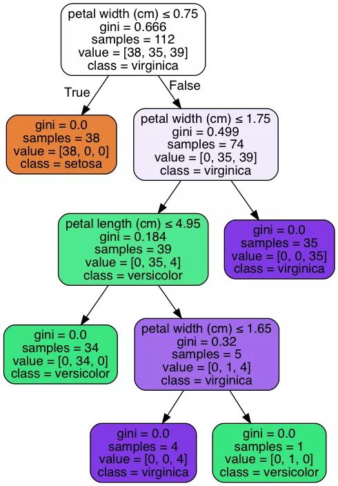
Decision Tree visualization, which is the resulting decision tree:
Anyang Kayo Amorphous Technology Co.,Ltd is located on the ancient city-Anyang. It was founded in 2011 that specializes in producing the magnetic ring of amorphous nanocrystalline and pays attention to scientific research highly,matches manufacture correspondingly and sets the design,development,production and sale in a body.Our major product is the magnetic ring of amorphous nanocrystalline and current transformer which is applied to the communication, home appliances, electric power, automobile and new energy extensively. We are highly praised by our customers for our good quality,high efficiency,excellent scheme,low cost and perfect sale service.
Fe-based amorphous Ribbon is an ultra-fine grain structure that has high permeability,high saturation magnetic induction,low loss and excelent stability. It can satisfy the requests of electronical products which is high frequency,large current,small volume and energy-saving.Especially it can replace the silicon steel,permalloy and ferrite and be used to all kinds of electronical products widely.
Amorphous Ribbon,Fe-Based Amorphous Ribbon,Low-Cost Amorphous Ribbon,Custom Fe-Based Amorphous Ribbon,Cheap Amorphous Ribbon
Anyang Kayo Amorphous Technology Co.,Ltd. , https://www.kayoamotech.com