In this series of articles, I would like to introduce the key algorithms behind the successful implementation of LTR, starting with linear regression, step by step to gradient boosTIng (together with different types of boosTIng algorithms), RankSVM and random forests.
LTR is first a regression problemFor this series of articles, as you learned in the previous article and in the documentation, I want to map LTR to a more general problem: regression. Regression problems require training a model to map a set of numerical features to a predicted value.
For example: What kind of data do you need to predict a company's profits? There may be historical public financial data at hand, including the number of employees, stock prices, earnings, and cash flow. Assuming that some company data is known, the function that your model is trained to predict for these variables (or a subset thereof) is the profit. For a new company, you can use this function to predict the company's profits.
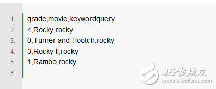
LTR is also a regression issue. You have a series of evaluation data on hand to measure the relevance level of a document to a query. Our relevance levels range from A to F. More common cases are values ​​ranging from 0 (completely uncorrelated) to 4 (very relevant). If we first consider a keyword search query, the following example:
When constructing a model to predict the rank as a time signal sorting function, the LTR becomes a regression problem. The recall in the relevance search, which we call the signal, represents any measure of the relationship between the query and the document; the more generic name is called the feature, but I personally recommend the long-term signal. One reason is that the signal is typically query-independent—that is, by measuring how much a keyword (or part of the query) is related to the document; some are measuring their relationship. So we can introduce other signals, including query-specific or document-specific, such as the publication date of an article, or some entity extracted from the query (such as "company name").
Take a look at the movie example above. You may suspect that there are 2 signals that rely on the query to help predict the correlation:
How many times has a search keyword appeared in the title attribute?
How many times has a search keyword appeared in the summary attribute?
Extending the above evaluation, you may get a regression training set as shown in the CSV file below, mapping the specific signal values ​​to levels:
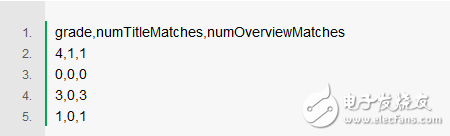
You can apply the regression process just like linear regression to predict the first column from other columns. It is also possible to build such a system on top of existing search engines like Solr or ElasTIcsearch.
I avoided a complicated question: how to get these evaluations? How do I know if a document is good or bad for a query? Understand user analysis? Expert analysis? This is usually the hardest to solve – and it's very relevant to a particular area! It is good to propose hypothetical data to build the model, but it is purely useless!
Linear regression LTRIf you have learned some statistics, you may already be familiar with linear regression. Linear regression defines a regression problem as a simple linear function. For example, in the LTR we call the first signal above (how many times a search keyword appears in the title attribute), and the second signal (how many times a search keyword appears in the summary attribute) is called o, our
![]()

The model can generate a function s, which scores the correlation as follows:
We can estimate the best fit coefficients c0, c1, c2, etc. and use the least squares fit method to predict our training data. I won't go into details here. The point is that we can find c0, c1, c2, etc. to minimize the error between the actual level g and the predicted value s(t, o). If you review linear algebra, you will find that it is like simple matrix mathematics.
You will be more satisfied with linear regression, including the decision to be another sorting signal, which we define as t*o. Or another signal, t2, is generally defined in practice as t^2 or log(t), or other best formula that you think is beneficial for correlation prediction. Next, you only need to use these values ​​as extra columns for the linear regression learning coefficients.
The design, testing, and evaluation of any model is a deeper art. If you want to know more, it is highly recommended to introduce statistical learning.
Linear regression LTR using sklearn
For a more intuitive experience, using Python's sklearn class library to implement regression is a convenient way. If you want to use the above data to try a simple LTR training set by linear regression, we can record the correlation level prediction value we tried as S, and the signal we see will predict the score and record it as X.
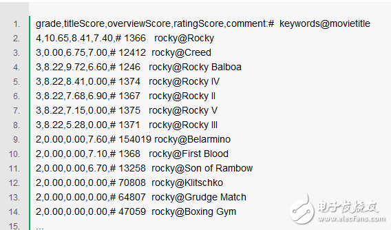
We will try some interesting things with some movie relevance data. Here is a correlation level data set for the search keyword "Rocky". Recall our judgement above and convert to a training set. Experience the real training set together (notes will help us understand the specific process). The three sorting signals we will examine include the TF*IDF score for the title, the TF*IDF score for the profile, and the rating for the movie spectator.
So go straight to the code section! The following code reads data from a CSV file into a numpy array; the array is two-dimensional, with the first dimension as the row and the second dimension as the column. In the comments below you can see how the very trendy array slices work:
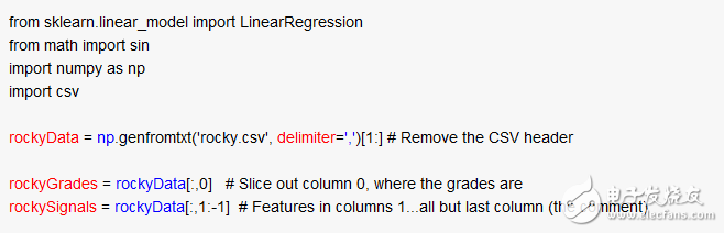
Not bad! We are ready for a simple linear regression. Here we use a classic method of judgment: the equation is more than the unknown! Therefore we need to use the least squares method to estimate the relationship between the characteristic rockySignals and the grade rockyGrades. Very simple, this is what numpy linear regression does:
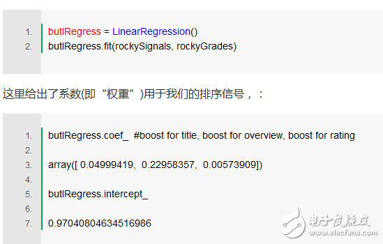
Pretty! The relevance is solved! (Really?) We can use these to build a sort function. We have learned what weights to use for the title and profile attributes respectively.
As of now, I have overlooked some of the things that we need to consider how to evaluate the match between the model and the data. At the end of this article, we just want to see how these models work in general. But it's not just assuming that the model is a good fit for training set data. It's always a good idea to roll back some data to test. The next blog post will introduce these topics separately.
Use the model to score the queryWe can build our own sorting function through these coefficients. This is done for descriptive purposes only. sk-learn's linear regression has a predictive method that evaluates the model as input, but building our own is more interesting:
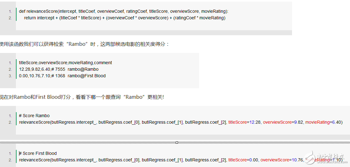
The results were scored by Rambo 3.670 and First Blood 3.671.
very close! First Blood is slightly better than Rambo. The reason is this - Rambo is an exact match, and First Blood is a Rambo movie prequel! So we shouldn't really make the model so credible, and there aren't so many examples to reach that level. More interesting is that the coefficient of the profile score is larger than the coefficient of the title score. So at least in this example our model shows that the more keywords mentioned in the introduction, the higher the final relevance tends to be. So far we have learned a good processing strategy to solve the relevance of the user!
Adding this model is more interesting, which is well understood and produces very plausible results; however, direct linear combinations of features are often not expected due to correlation applications. Due to the lack of such reasons, as the counterparts of Flax said, the direct weighted boosTIng also fell short of expectations.
why? details make a difference!From the previous examples, it can be found that some very related movies do have a high TF*IDF correlation score, but the model tends to be more closely related to the summary field. In fact, when the title matches and when the summary matches, it depends on other factors.
In many problems, the scores of relevance levels and title and summary attributes are not a simple linear relationship, but contextual. If you want to search for a title directly, then the title will definitely match more; but it is not easy to determine if you want to search for the title, or the category, or the actors of the movie, or even other attributes.
In other words, the relevance issue does not seem to be a purely optimal problem:
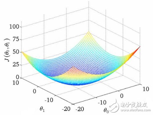
The relevance in practice is more complicated. There is no magical optimal solution. It is better to say that many local optimisations depend on many other factors! why? In other words, the relevance looks like this:
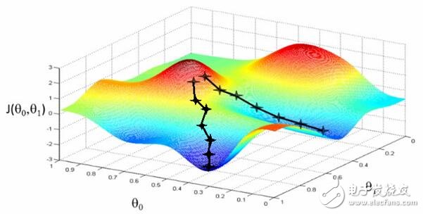
It is conceivable that these figures (dry goods in the Wu Enda machine learning course) are used to show “related errors†– how far away we are from the scores we are learning. The mapping of the two theta variables represents the relevance score for the title and the abstract. The first picture has a single optimal value where the "correlation error" is minimal - an ideal weight setting applies to both queries. The second is more practical: undulating, context-sensitive local minimum. Sometimes related to a very high title weight value, or a very low title weight!
Basic Physics Experiment Instrument Series
Basic physics experiment instrument series, used in physics laboratories of colleges and universities.
Basic Physics Experiment Instrument,Light And Optical Instruments,Optical Viewing Instrument,Microscope Light Source Instrument
Yuheng Optics Co., Ltd.(Changchun) , https://www.yhenoptics.com